本文仅供学习使用
本文参考:
B站:CLEAR_LAB
笔者带更新-运动学
课程主讲教师:
Prof. Wei Zhang
南科大高等机器人控制课 Ch08 Rigid Body Dynamics
- 1. Spatial Vecocity
- 1.1 Spatial vs. Conventional Accel
- 1.2 Plueker Coordinate System and Basis Vectors
- 1.3 Work with Moving Reference Frame
- 1.4 Derivative of Adjoint
- 1.4.1 Spatial Cross Product
- 1.4.2 Spatial Acceleration with Moving Reference Frame
- 2. Spatial Force(Wrench)
- 2.1 Spatial Force in Pluecker Coordinate Systems
- 2.2 Wrench-Twist Pair and Power
- 2.3 Joint Torque
- 3. Spatial Momentum
- 3.1 Rotational Interial
- 3.2 Change Reference for Momentum
- 3.3 Spatial Inertia
- 4. Newton-Euler Equation using Spatial Vectors
- 4.1 Cross Product for Spatial Force and Momentum
- 4.2 Newton-Euler Equation
- 4.3 Derivations of Newton-Euler Equation
1. Spatial Vecocity
Given a rigid body with spatial velocity
V
=
(
ω
⃗
,
v
⃗
)
\mathcal{V} =\left( \vec{\omega},\vec{v} \right)
V=(ω,v) , its spatial acceleration (coordinate-free)
A
=
V
˙
=
[
ω
⃗
˙
v
⃗
˙
O
]
,
A
=
lim
δ
→
0
V
(
t
+
δ
)
−
V
(
t
)
δ
\mathcal{A} =\dot{\mathcal{V}}=\left[ \begin{array}{c} \dot{\vec{\omega}}\\ \dot{\vec{v}}_{\mathrm{O}}\\ \end{array} \right] ,\mathcal{A} =\underset{\delta \rightarrow 0}{\lim}\frac{\mathcal{V} \left( t+\delta \right) -\mathcal{V} \left( t \right)}{\delta}
A=V˙=[ω˙v˙O],A=δ→0limδV(t+δ)−V(t)
Recall that:
v
⃗
O
\vec{v}_{\mathrm{O}}
vO i sthe velocity of the body-fixed particle coincident with frame origin
o
o
o at the current time
t
t
t
Note : ω ⃗ ˙ \dot{\vec{\omega}} ω˙ is the angular acceleration of the body
v ⃗ ˙ O \dot{\vec{v}}_{\mathrm{O}} v˙O is not the acceleration of any body-fixed point ! v ⃗ O = R ⃗ ˙ q ( t ) , v ⃗ ˙ O ≠ R ⃗ ¨ q ( t ) \vec{v}_{\mathrm{O}}=\dot{\vec{R}}_q\left( t \right) ,\dot{\vec{v}}_{\mathrm{O}}\ne \ddot{\vec{R}}_q\left( t \right) vO=R˙q(t),v˙O=R¨q(t)
In face, v ⃗ ˙ O \dot{\vec{v}}_{\mathrm{O}} v˙O gives the rate of change in stream velocity of body-fixed particles passing through o o o
1.1 Spatial vs. Conventional Accel
Suppose
R
⃗
q
(
t
)
\vec{R}_q\left( t \right)
Rq(t) is the body fixed particle coincides with
o
o
o at time
t
t
t
So by definition , we have
v
⃗
O
(
t
)
=
R
⃗
˙
q
(
t
)
\vec{v}_{\mathrm{O}}\left( t \right) =\dot{\vec{R}}_q\left( t \right)
vO(t)=R˙q(t) , however
v
⃗
˙
O
≠
R
⃗
¨
q
(
t
)
\dot{\vec{v}}_{\mathrm{O}}\ne \ddot{\vec{R}}_q\left( t \right)
v˙O=R¨q(t) , where
R
⃗
¨
q
(
t
)
\ddot{\vec{R}}_q\left( t \right)
R¨q(t) is the conventional acceleration of the body-fixed point
q
q
q
At time
t
t
t :
R
⃗
q
(
t
)
=
0
\vec{R}_q\left( t \right) =0
Rq(t)=0 ,
v
⃗
O
(
t
)
=
R
⃗
˙
q
(
t
)
\vec{v}_{\mathrm{O}}\left( t \right) =\dot{\vec{R}}_q\left( t \right)
vO(t)=R˙q(t)
At time
t
+
δ
t+\delta
t+δ :
R
⃗
q
′
(
t
)
=
0
\vec{R}_{q^{\prime}}\left( t \right) =0
Rq′(t)=0 ,
v
⃗
O
(
t
+
δ
)
=
R
⃗
˙
q
′
(
t
+
δ
)
≠
R
⃗
˙
q
(
t
+
δ
)
\vec{v}_{\mathrm{O}}\left( t+\delta \right) =\,\,\dot{\vec{R}}_{q^{\prime}}\left( t+\delta \right) \ne \dot{\vec{R}}_q\left( t+\delta \right)
vO(t+δ)=R˙q′(t+δ)=R˙q(t+δ) ——
q
′
q^{\prime}
q′ another body-fixed particle
- Note : q q q and q ′ q^{\prime} q′ are different points, lim δ → 0 v ⃗ O ( t ) = v ⃗ O ( t + δ ) − v ⃗ O ( t ) δ = R ⃗ ˙ q ′ ( t + δ ) − R ⃗ q ( t ) δ \underset{\delta \rightarrow 0}{\lim}\vec{v}_{\mathrm{O}}\left( t \right) =\frac{\vec{v}_{\mathrm{O}}\left( t+\delta \right) -\vec{v}_{\mathrm{O}}\left( t \right)}{\delta}=\frac{\dot{\vec{R}}_{q^{\prime}}\left( t+\delta \right) -\vec{R}_q\left( t \right)}{\delta} δ→0limvO(t)=δvO(t+δ)−vO(t)=δR˙q′(t+δ)−Rq(t)
实际上只需考虑Twist最开始的定义,即速度 v ⃗ O \vec{v}_{\mathrm{O}} vO 并不是某一点的速度,而是考虑相对坐标系原点而言的虚拟点在该角速度下的瞬时速度( R ⃗ ˙ q ( t ) = v ⃗ O ( t ) + ω ⃗ ( t ) × R ⃗ q ( t ) \dot{\vec{R}}_q\left( t \right) =\vec{v}_{\mathrm{O}}\left( t \right) +\vec{\omega}\left( t \right) \times \vec{R}_q\left( t \right) R˙q(t)=vO(t)+ω(t)×Rq(t)),而与该坐标系所代表的真实点的运动无关( R ⃗ q ( t ) \vec{R}_q\left( t \right) Rq(t) is the body fixed particle coincides with o o o at time t t t),即为:
R ⃗ ¨ q ( t ) = v ⃗ ˙ O ( t ) + ω ⃗ ˙ ( t ) × R ⃗ q ( t ) ↗ 0 + ω ⃗ ( t ) × R ⃗ ˙ q ( t ) = v ⃗ ˙ O ( t ) + ω ⃗ ( t ) × R ⃗ ˙ q ( t ) \ddot{\vec{R}}_q\left( t \right) =\dot{\vec{v}}_{\mathrm{O}}\left( t \right) +\dot{\vec{\omega}}\left( t \right) \times \vec{R}_q\left( t \right) _{\nearrow 0}+\vec{\omega}\left( t \right) \times \dot{\vec{R}}_q\left( t \right) =\dot{\vec{v}}_{\mathrm{O}}\left( t \right) +\vec{\omega}\left( t \right) \times \dot{\vec{R}}_q\left( t \right) R¨q(t)=v˙O(t)+ω˙(t)×Rq(t)↗0+ω(t)×R˙q(t)=v˙O(t)+ω(t)×R˙q(t)
1.2 Plueker Coordinate System and Basis Vectors
按照向量的本质理解即可,这也是笔者为啥不是很喜欢旋量的原因。
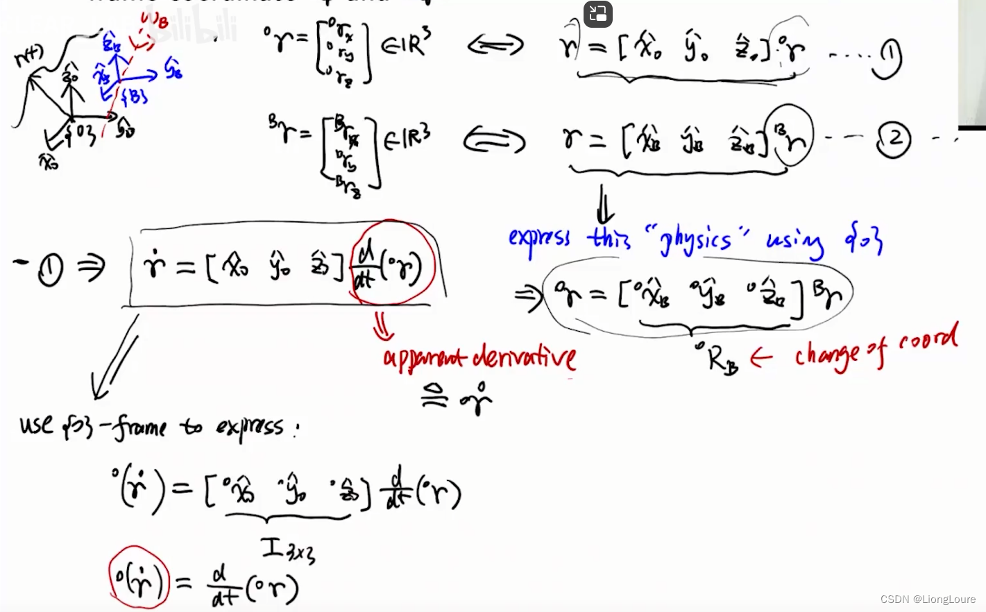
Recall coordinate-free concept: let R ⃗ ∈ R 3 \vec{R}\in \mathbb{R} ^3 R∈R3 be a free vector with { O } \left\{ O \right\} {O} and { B } \left\{ B \right\} {B} frame coordinate R ⃗ O \vec{R}^O RO and R ⃗ B \vec{R}^B RB
矢量的变换:
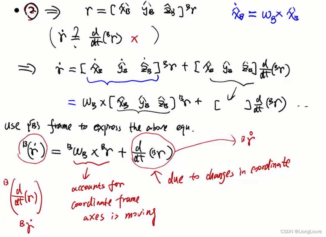
旋量的变换:
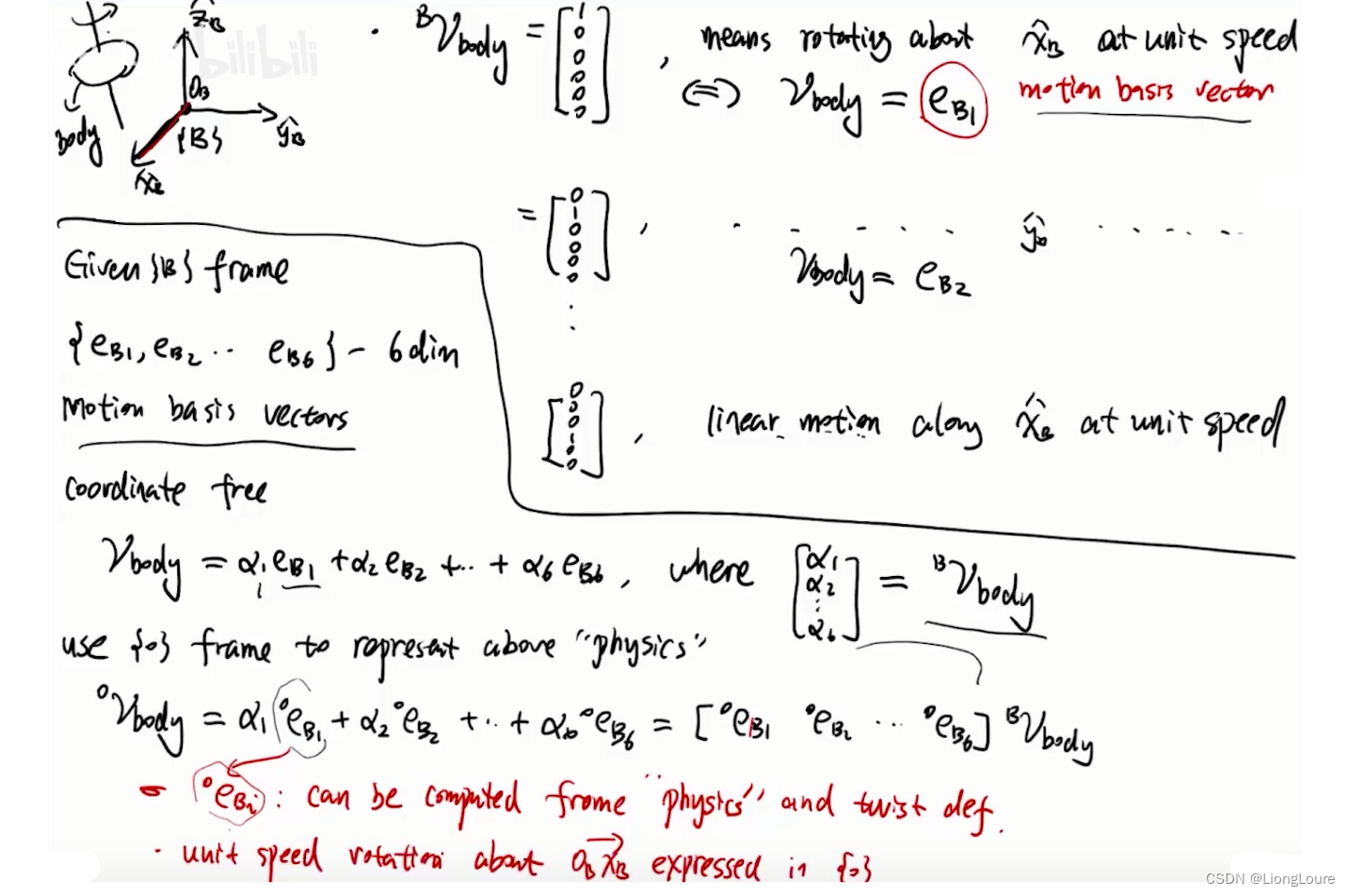
[
e
B
1
O
e
B
2
O
e
B
3
O
e
B
4
O
e
B
4
O
e
B
5
O
]
6
×
6
=
[
X
B
O
]
=
[
A
d
[
T
B
O
]
]
\left[ \begin{array}{l} e_{\mathrm{B}1}^{O}& e_{\mathrm{B}2}^{O}& e_{\mathrm{B}3}^{O}& e_{\mathrm{B}4}^{O}& e_{\mathrm{B}4}^{O}& e_{\mathrm{B}5}^{O}\\ \end{array} \right] _{6\times 6}=\left[ X_{\mathrm{B}}^{O} \right] =\left[ Ad_{\left[ T_{\mathrm{B}}^{O} \right]} \right]
[eB1OeB2OeB3OeB4OeB4OeB5O]6×6=[XBO]=[Ad[TBO]]
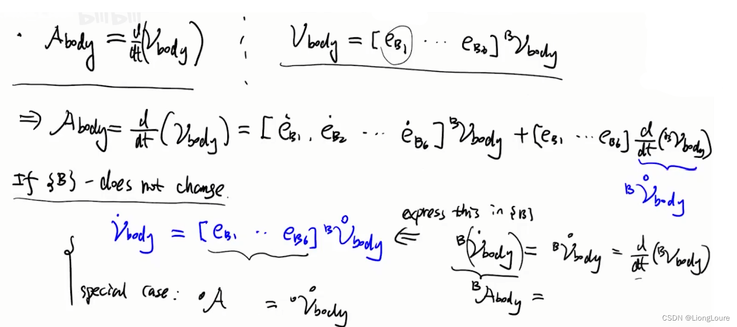

1.3 Work with Moving Reference Frame
Now let’s work with { O } \left\{ O \right\} {O} frame to find the derivative —— we need to compute : [ e ˙ B 1 O e ˙ B 2 O e ˙ B 3 O e ˙ B 4 O e ˙ B 4 O e ˙ B 5 O ] 6 × 6 = [ X ˙ B O ] = d d t [ A d [ T B O ] ] \left[ \begin{array}{l} \dot{e}_{\mathrm{B}1}^{O}& \dot{e}_{\mathrm{B}2}^{O}& \dot{e}_{\mathrm{B}3}^{O}& \dot{e}_{\mathrm{B}4}^{O}& \dot{e}_{\mathrm{B}4}^{O}& \dot{e}_{\mathrm{B}5}^{O}\\ \end{array} \right] _{6\times 6}=\left[ \dot{X}_{\mathrm{B}}^{O} \right] =\frac{\mathrm{d}}{\mathrm{d}t}\left[ Ad_{\left[ T_{\mathrm{B}}^{O} \right]} \right] [e˙B1Oe˙B2Oe˙B3Oe˙B4Oe˙B4Oe˙B5O]6×6=[X˙BO]=dtd[Ad[TBO]]
Let’s denote : [ T B O ] = ( [ Q ] , R ⃗ ) ⇒ d d t ( [ [ Q ] 0 R ⃗ ~ [ Q ] [ Q ] ] ) = [ [ Q ˙ ] 0 ( R ⃗ ~ [ Q ] ) ′ [ Q ˙ ] ] \left[ T_{\mathrm{B}}^{O} \right] =\left( \left[ Q \right] ,\vec{R} \right) \Rightarrow \frac{\mathrm{d}}{\mathrm{d}t}\left( \left[ \begin{matrix} \left[ Q \right]& 0\\ \tilde{\vec{R}}\left[ Q \right]& \left[ Q \right]\\ \end{matrix} \right] \right) =\left[ \begin{matrix} \left[ \dot{Q} \right]& 0\\ \left( \tilde{\vec{R}}\left[ Q \right] \right) ^{\prime}& \left[ \dot{Q} \right]\\ \end{matrix} \right] [TBO]=([Q],R)⇒dtd([[Q]R~[Q]0[Q]])= [Q˙](R~[Q])′0[Q˙]
{ B } \left\{ B \right\} {B} frame has instantaneous velocity V B = [ ω ⃗ v ⃗ O ] \mathcal{V} _B=\left[ \begin{array}{c} \vec{\omega}\\ \vec{v}_{\mathrm{O}}\\ \end{array} \right] VB=[ωvO]
1.4 Derivative of Adjoint
Note : [ Q ˙ ] = ω ⃗ × [ Q ] , R ⃗ ˙ = v ⃗ O + ω ⃗ × R ⃗ , [ Q ] ω ⃗ ~ = [ Q ] ω ⃗ ~ [ Q ] T , ω ⃗ 1 × ω ⃗ 2 ~ = ω ⃗ ~ 1 ω ⃗ ~ 2 − ω ⃗ ~ 2 ω ⃗ ~ 1 \left[ \dot{Q} \right] =\vec{\omega}\times \left[ Q \right] ,\dot{\vec{R}}=\vec{v}_{\mathrm{O}}+\vec{\omega}\times \vec{R},\widetilde{\left[ Q \right] \vec{\omega}}=\left[ Q \right] \tilde{\vec{\omega}}\left[ Q \right] ^{\mathrm{T}},\widetilde{\vec{\omega}_1\times \vec{\omega}_2}=\tilde{\vec{\omega}}_1\tilde{\vec{\omega}}_2-\tilde{\vec{\omega}}_2\tilde{\vec{\omega}}_1 [Q˙]=ω×[Q],R˙=vO+ω×R,[Q]ω =[Q]ω~[Q]T,ω1×ω2 =ω~1ω~2−ω~2ω~1(Jacobi’s Identity)
After some computation :
d
d
t
[
A
d
[
T
B
O
]
]
=
[
ω
⃗
~
0
v
⃗
~
O
ω
⃗
~
]
[
A
d
[
T
B
O
]
]
=
[
X
˙
B
O
]
\frac{\mathrm{d}}{\mathrm{d}t}\left[ Ad_{\left[ T_{\mathrm{B}}^{O} \right]} \right] =\left[ \begin{matrix} \tilde{\vec{\omega}}& 0\\ \tilde{\vec{v}}_{\mathrm{O}}& \tilde{\vec{\omega}}\\ \end{matrix} \right] \left[ Ad_{\left[ T_{\mathrm{B}}^{O} \right]} \right] =\left[ \dot{X}_{\mathrm{B}}^{O} \right]
dtd[Ad[TBO]]=[ω~v~O0ω~][Ad[TBO]]=[X˙BO]
Define : [ ω ⃗ ~ 0 v ⃗ ~ O ω ⃗ ~ ] = V ~ B \left[ \begin{matrix} \tilde{\vec{\omega}}& 0\\ \tilde{\vec{v}}_{\mathrm{O}}& \tilde{\vec{\omega}}\\ \end{matrix} \right] =\tilde{\mathcal{V}}_B [ω~v~O0ω~]=V~B
{ [ Q ˙ B O ] = ω ⃗ ~ B [ Q B O ] [ X ˙ B O ] = V ~ B [ X ˙ B O ] \begin{cases} \left[ \dot{Q}_{\mathrm{B}}^{O} \right] =\tilde{\vec{\omega}}_B\left[ Q_{\mathrm{B}}^{O} \right]\\ \left[ \dot{X}_{\mathrm{B}}^{O} \right] =\tilde{\mathcal{V}}_B\left[ \dot{X}_{\mathrm{B}}^{O} \right]\\ \end{cases} ⎩ ⎨ ⎧[Q˙BO]=ω~B[QBO][X˙BO]=V~B[X˙BO]
In coordinate free: e ˙ B 1 O = V ~ B e B 1 O \dot{e}_{\mathrm{B}1}^{O}=\tilde{\mathcal{V}}_Be_{\mathrm{B}1}^{O} e˙B1O=V~BeB1O
1.4.1 Spatial Cross Product
Given two spatial velocities(twists)
V
1
\mathcal{V} _1
V1 and
V
2
\mathcal{V} _2
V2 , their spatial product is
V
1
×
V
2
=
[
ω
⃗
1
v
⃗
1
O
]
×
[
ω
⃗
2
v
⃗
2
O
]
=
[
ω
⃗
1
×
ω
⃗
2
ω
⃗
1
×
v
⃗
2
O
+
v
⃗
1
O
×
ω
⃗
2
]
\mathcal{V} _1\times \mathcal{V} _2=\left[ \begin{array}{c} \vec{\omega}_1\\ {\vec{v}_1}_{\mathrm{O}}\\ \end{array} \right] \times \left[ \begin{array}{c} \vec{\omega}_2\\ {\vec{v}_2}_{\mathrm{O}}\\ \end{array} \right] =\left[ \begin{array}{c} \vec{\omega}_1\times \vec{\omega}_2\\ \vec{\omega}_1\times {\vec{v}_2}_{\mathrm{O}}+{\vec{v}_1}_{\mathrm{O}}\times \vec{\omega}_2\\ \end{array} \right]
V1×V2=[ω1v1O]×[ω2v2O]=[ω1×ω2ω1×v2O+v1O×ω2]
Matrix representation : V 1 × V 2 = V ~ 1 V 2 , V ~ 1 = [ ω ⃗ ~ 1 0 v ⃗ ~ 1 O ω ⃗ ~ 1 ] \mathcal{V} _1\times \mathcal{V} _2=\tilde{\mathcal{V}}_1\mathcal{V} _2,\tilde{\mathcal{V}}_1=\left[ \begin{matrix} \tilde{\vec{\omega}}_1& 0\\ {\tilde{\vec{v}}_1}_{\mathrm{O}}& \tilde{\vec{\omega}}_1\\ \end{matrix} \right] V1×V2=V~1V2,V~1=[ω~1v~1O0ω~1]
Roughly speaking, when a motion
V
\mathcal{V}
V is moving with a spatial velocity
Z
\mathcal{Z}
Z (e.g. it is attached to a moving frame) but is otherwise not changing , then
V
˙
=
Z
×
V
\dot{\mathcal{V}}=\mathcal{Z} \times \mathcal{V}
V˙=Z×V
- Propertries
Assume A is moving wrt
O
O
O with velocity
V
A
\mathcal{V} _{\mathrm{A}}
VA :
[
X
˙
A
O
]
=
V
~
A
O
[
X
A
O
]
\left[ \dot{X}_{\mathrm{A}}^{O} \right] =\tilde{\mathcal{V}}_{\mathrm{A}}^{O}\left[ X_{\mathrm{A}}^{O} \right]
[X˙AO]=V~AO[XAO]
[
X
]
V
~
=
[
X
]
V
~
[
X
]
T
\widetilde{\left[ X \right] \mathcal{V} }=\left[ X \right] \tilde{\mathcal{V}}\left[ X \right] ^{\mathrm{T}}
[X]V
=[X]V~[X]T for any transformation
[
X
]
\left[ X \right]
[X] and twist
V
\mathcal{V}
V
1.4.2 Spatial Acceleration with Moving Reference Frame
Consider a body with velocity
V
B
o
d
y
\mathcal{V} _{\mathrm{Body}}
VBody (wrt inertia frame), and
V
B
o
d
y
O
\mathcal{V} _{\mathrm{Body}}^{O}
VBodyO and
V
B
o
d
y
B
\mathcal{V} _{\mathrm{Body}}^{B}
VBodyB be its Plueker coordinates wrt
{
O
}
\left\{ O \right\}
{O} and
{
B
}
\left\{ B \right\}
{B} :
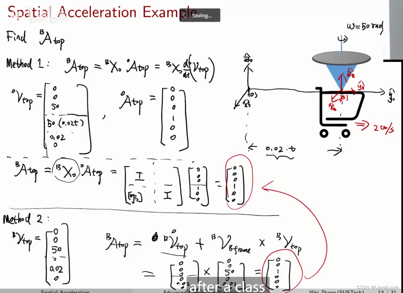
A
B
o
d
y
B
=
d
d
t
(
V
B
o
d
y
B
)
+
V
~
B
O
B
V
B
o
d
y
B
\mathcal{A} _{\mathrm{Body}}^{B}=\frac{\mathrm{d}}{\mathrm{d}t}\left( \mathcal{V} _{\mathrm{Body}}^{B} \right) +\tilde{\mathcal{V}}_{\mathrm{BO}}^{B}\mathcal{V} _{\mathrm{Body}}^{B}
ABodyB=dtd(VBodyB)+V~BOBVBodyB
A
B
o
d
y
O
=
[
X
B
O
]
A
B
o
d
y
B
\mathcal{A} _{\mathrm{Body}}^{O}=\left[ X_{\mathrm{B}}^{O} \right] \mathcal{A} _{\mathrm{Body}}^{B}
ABodyO=[XBO]ABodyB
A B o d y O = d d t ( V B o d y O ) = d d t ( [ X B O ] V B o d y B ) = [ X ˙ B O ] V B o d y B + [ X B O ] V ˙ B o d y B = V ~ B O [ X B O ] V B o d y B + [ X B O ] V ˙ B o d y B = [ X B O ] ( [ X O B ] V ~ B O [ X B O ] V B o d y B + V ˙ B o d y B ) = [ X B O ] ( [ X O B ] V B O ~ V B o d y B + V ˙ B o d y B ) = [ X B O ] ( V ~ B O B V B o d y B + V ˙ B o d y B ) = [ X B O ] A B o d y B \mathcal{A} _{\mathrm{Body}}^{O}=\frac{\mathrm{d}}{\mathrm{d}t}\left( \mathcal{V} _{\mathrm{Body}}^{O} \right) =\frac{\mathrm{d}}{\mathrm{d}t}\left( \left[ X_{\mathrm{B}}^{O} \right] \mathcal{V} _{\mathrm{Body}}^{B} \right) =\left[ \dot{X}_{\mathrm{B}}^{O} \right] \mathcal{V} _{\mathrm{Body}}^{B}+\left[ X_{\mathrm{B}}^{O} \right] \dot{\mathcal{V}}_{\mathrm{Body}}^{B}=\tilde{\mathcal{V}}_{\mathrm{B}}^{O}\left[ X_{\mathrm{B}}^{O} \right] \mathcal{V} _{\mathrm{Body}}^{B}+\left[ X_{\mathrm{B}}^{O} \right] \dot{\mathcal{V}}_{\mathrm{Body}}^{B}=\left[ X_{\mathrm{B}}^{O} \right] \left( \left[ X_{\mathrm{O}}^{B} \right] \tilde{\mathcal{V}}_{\mathrm{B}}^{O}\left[ X_{\mathrm{B}}^{O} \right] \mathcal{V} _{\mathrm{Body}}^{B}+\dot{\mathcal{V}}_{\mathrm{Body}}^{B} \right) =\left[ X_{\mathrm{B}}^{O} \right] \left( \widetilde{\left[ X_{\mathrm{O}}^{B} \right] \mathcal{V} _{\mathrm{B}}^{O}}\mathcal{V} _{\mathrm{Body}}^{B}+\dot{\mathcal{V}}_{\mathrm{Body}}^{B} \right) =\left[ X_{\mathrm{B}}^{O} \right] \left( \tilde{\mathcal{V}}_{\mathrm{BO}}^{B}\mathcal{V} _{\mathrm{Body}}^{B}+\dot{\mathcal{V}}_{\mathrm{Body}}^{B} \right) =\left[ X_{\mathrm{B}}^{O} \right] \mathcal{A} _{\mathrm{Body}}^{B} ABodyO=dtd(VBodyO)=dtd([XBO]VBodyB)=[X˙BO]VBodyB+[XBO]V˙BodyB=V~BO[XBO]VBodyB+[XBO]V˙BodyB=[XBO]([XOB]V~BO[XBO]VBodyB+V˙BodyB)=[XBO]([XOB]VBO VBodyB+V˙BodyB)=[XBO](V~BOBVBodyB+V˙BodyB)=[XBO]ABodyB
EXAMPLE:
2. Spatial Force(Wrench)
Consider a rigid body with many forces on it and fix an arbitrary point
O
O
O in space

The net effect of these forces can be expressed as:
- A force f f f , acting along a line passing through O O O —— f ⃗ = ∑ f ⃗ i i \vec{f}=\sum{\vec{f}_{\mathrm{i}}}_{\mathrm{i}} f=∑fii
- A moment m ⃗ O \vec{m}_{\mathrm{O}} mO about point O O O —— m ⃗ O = ∑ R ⃗ P i O × f ⃗ i \vec{m}_{\mathrm{O}}=\sum{\vec{R}_{\mathrm{Pi}}^{O}\times \vec{f}_{\mathrm{i}}} mO=∑RPiO×fi
Spatial Force(Wrench) : is given by the 6D vector
F = [ m ⃗ O f ⃗ ] \mathcal{F} =\left[ \begin{array}{c} \vec{m}_{\mathrm{O}}\\ \vec{f}\\ \end{array} \right] F=[mOf]
What is we choose reference point to
Q
Q
Q?
m
⃗
Q
=
∑
R
⃗
P
i
Q
×
f
⃗
i
=
∑
(
R
⃗
O
Q
+
R
⃗
P
i
O
)
×
f
⃗
i
=
m
⃗
O
+
∑
R
⃗
O
Q
×
f
⃗
i
\vec{m}_{\mathrm{Q}}=\sum{\vec{R}_{\mathrm{Pi}}^{Q}\times \vec{f}_{\mathrm{i}}}=\sum{\left( \vec{R}_{\mathrm{O}}^{Q}+\vec{R}_{\mathrm{Pi}}^{O} \right) \times \vec{f}_{\mathrm{i}}}=\vec{m}_{\mathrm{O}}+\sum{\vec{R}_{\mathrm{O}}^{Q}\times \vec{f}_{\mathrm{i}}}
mQ=∑RPiQ×fi=∑(ROQ+RPiO)×fi=mO+∑ROQ×fi
2.1 Spatial Force in Pluecker Coordinate Systems
Given a frame { A } \left\{ A \right\} {A}, the Plueker coordinate of a spatial force F \mathcal{F} F is given by F A = [ m ⃗ O A f ⃗ A ] \mathcal{F} ^A=\left[ \begin{array}{c} \vec{m}_{\mathrm{O}}^{A}\\ \vec{f}^A\\ \end{array} \right] FA=[mOAfA]
Coordinate transform :
{
f
⃗
A
=
[
Q
B
A
]
f
⃗
B
m
⃗
O
A
=
[
Q
B
A
]
m
⃗
O
B
+
R
⃗
B
A
×
[
Q
B
A
]
f
⃗
B
⇒
F
A
=
[
X
B
A
]
T
F
B
=
[
X
B
A
]
∗
F
B
\begin{cases} \vec{f}^A=\left[ Q_{\mathrm{B}}^{A} \right] \vec{f}^B\\ \vec{m}_{\mathrm{O}}^{A}=\left[ Q_{\mathrm{B}}^{A} \right] \vec{m}_{\mathrm{O}}^{B}+\vec{R}_{\mathrm{B}}^{A}\times \left[ Q_{\mathrm{B}}^{A} \right] \vec{f}^B\\ \end{cases}\Rightarrow \mathcal{F} ^A=\left[ X_{\mathrm{B}}^{A} \right] ^{\mathrm{T}}\mathcal{F} ^B=\left[ X_{\mathrm{B}}^{A} \right] ^*\mathcal{F} ^B
{fA=[QBA]fBmOA=[QBA]mOB+RBA×[QBA]fB⇒FA=[XBA]TFB=[XBA]∗FB
2.2 Wrench-Twist Pair and Power
Recall that for a point mass with linear velocity v ⃗ \vec{v} v and a linear force f ⃗ \vec{f} f . Then we know that the power (instantaneous work done by f ⃗ \vec{f} f ) is given by : f ⃗ ⋅ v ⃗ = f ⃗ T v ⃗ \vec{f}\cdot \vec{v}=\vec{f}^{\mathrm{T}}\vec{v} f⋅v=fTv
This relation can be generalized to spatial force (i.e. wrench) and spatial velocity (i.e. twist)
Suppose a rigid body has a twist
V
A
=
(
ω
⃗
A
,
v
⃗
O
A
)
\mathcal{V} ^A=\left( \vec{\omega}^A,\vec{v}_{\mathrm{O}}^{A} \right)
VA=(ωA,vOA) and a wrench
F
A
=
(
m
⃗
O
A
,
f
⃗
A
)
\mathcal{F} ^A=\left( \vec{m}_{\mathrm{O}}^{A},\vec{f}^A \right)
FA=(mOA,fA) acts on the body. Then the power is simply
P
=
(
V
A
)
T
F
A
=
(
F
A
)
T
V
A
=
(
ω
⃗
A
)
T
m
⃗
O
A
+
(
v
⃗
O
A
)
T
f
⃗
A
P=\left( \mathcal{V} ^A \right) ^{\mathrm{T}}\mathcal{F} ^A=\left( \mathcal{F} ^A \right) ^{\mathrm{T}}\mathcal{V} ^A=\left( \vec{\omega}^A \right) ^{\mathrm{T}}\vec{m}_{\mathrm{O}}^{A}+\left( \vec{v}_{\mathrm{O}}^{A} \right) ^{\mathrm{T}}\vec{f}^A
P=(VA)TFA=(FA)TVA=(ωA)TmOA+(vOA)TfA
2.3 Joint Torque
Consider a link attached to a 1-dof joint(r.g. revolute or prismatic). be the screw axis of the joint. Then the power produced by the joint is V = S ^ θ ˙ \mathcal{V} =\hat{\mathcal{S}}\dot{\theta} V=S^θ˙
F \mathcal{F} F be the wrench provided by the joint. Then the power produced by the joint is P = ( V ) T F = ( S ^ θ ˙ ) T F = ( S ^ T F ) θ ˙ = τ θ ˙ P=\left( \mathcal{V} \right) ^{\mathrm{T}}\mathcal{F} =\left( \hat{\mathcal{S}}\dot{\theta} \right) ^{\mathrm{T}}\mathcal{F} =\left( \hat{\mathcal{S}}^{\mathrm{T}}\mathcal{F} \right) \dot{\theta}=\tau \dot{\theta} P=(V)TF=(S^θ˙)TF=(S^TF)θ˙=τθ˙
τ = S ^ T F = F T S ^ \tau =\hat{\mathcal{S}}^{\mathrm{T}}\mathcal{F} =\mathcal{F} ^{\mathrm{T}}\hat{\mathcal{S}} τ=S^TF=FTS^ is the projection of the wrench onto the screw axis, i.e. the effective part of the wrench
Often times, τ \tau τ is referred to as joint “torque” or generalized force
3. Spatial Momentum
笔者待整理: 链接
3.1 Rotational Interial
- Recall momentum for point mass:
笔者待整理: 链接
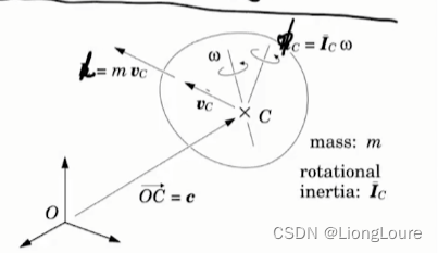
H = [ h ⃗ p ⃗ ] ∈ R 6 \mathcal{H} =\left[ \begin{array}{c} \vec{h}\\ \vec{p}\\ \end{array} \right] \in \mathbb{R} ^6 H=[hp]∈R6
3.2 Change Reference for Momentum
- Spatial momentum transforms in the same way as spatial forces:
H A = [ X C A ] ∗ H C \mathcal{H} ^A=\left[ X_{\mathrm{C}}^{A} \right] ^*\mathcal{H} ^C HA=[XCA]∗HC
H C = [ h ⃗ B o d y / C C p ⃗ C ] , H A = [ h ⃗ A A p ⃗ A ] = [ [ Q C A ] h ⃗ B o d y / C C − R ⃗ ~ C A [ Q C A ] p ⃗ C [ Q C A ] p ⃗ C ] = [ [ Q C A ] − R ⃗ ~ C A [ Q C A ] 0 [ Q C A ] ] [ h ⃗ B o d y / C C p ⃗ C ] = [ X C A ] ∗ [ h ⃗ B o d y / C C p ⃗ C ] \mathcal{H} ^C=\left[ \begin{array}{c} \vec{h}_{\mathrm{Body}/\mathrm{C}}^{C}\\ \vec{p}^C\\ \end{array} \right] ,\mathcal{H} ^A=\left[ \begin{array}{c} \vec{h}_{\mathrm{A}}^{A}\\ \vec{p}^A\\ \end{array} \right] =\left[ \begin{array}{c} \left[ Q_{\mathrm{C}}^{A} \right] \vec{h}_{\mathrm{Body}/\mathrm{C}}^{C}-\tilde{\vec{R}}_{\mathrm{C}}^{A}\left[ Q_{\mathrm{C}}^{A} \right] \vec{p}^C\\ \left[ Q_{\mathrm{C}}^{A} \right] \vec{p}^C\\ \end{array} \right] =\left[ \begin{matrix} \left[ Q_{\mathrm{C}}^{A} \right]& -\tilde{\vec{R}}_{\mathrm{C}}^{A}\left[ Q_{\mathrm{C}}^{A} \right]\\ 0& \left[ Q_{\mathrm{C}}^{A} \right]\\ \end{matrix} \right] \left[ \begin{array}{c} \vec{h}_{\mathrm{Body}/\mathrm{C}}^{C}\\ \vec{p}^C\\ \end{array} \right] =\left[ X_{\mathrm{C}}^{A} \right] ^*\left[ \begin{array}{c} \vec{h}_{\mathrm{Body}/\mathrm{C}}^{C}\\ \vec{p}^C\\ \end{array} \right] HC=[hBody/CCpC],HA=[hAApA]=[[QCA]hBody/CC−R~CA[QCA]pC[QCA]pC]=[[QCA]0−R~CA[QCA][QCA]][hBody/CCpC]=[XCA]∗[hBody/CCpC]
3.3 Spatial Inertia
Inertia of a rigid body defines linear relationship between velocity and momentum
Spacial inertia
I
\mathcal{I}
I is the one such that
H
=
I
V
\mathcal{H} =\mathcal{I} \mathcal{V}
H=IV
Let
{
M
}
\left\{ M \right\}
{M} be a frame whose origin coincide with CoM. Then
I
B
o
d
y
/
C
o
M
M
=
[
I
B
o
d
y
/
C
o
M
M
0
0
m
t
o
t
a
l
E
3
×
3
]
G
\mathcal{I} _{\mathrm{Body}/\mathrm{CoM}}^{M}=\left[ \begin{matrix} I_{\mathrm{Body}/\mathrm{CoM}}^{M}& 0\\ 0& m_{\mathrm{total}}E_{3\times 3}\\ \end{matrix} \right] G
IBody/CoMM=[IBody/CoMM00mtotalE3×3]G
- Spatial inertia wrt another frame
{
F
}
\left\{ F \right\}
{F}:
I F = [ X M F ] ∗ I M [ X F M ] \mathcal{I} ^F=\left[ X_{\mathrm{M}}^{F} \right] ^*\mathcal{I} ^M\left[ X_{\mathrm{F}}^{M} \right] IF=[XMF]∗IM[XFM]
Special case : [ Q F M ] = E 3 × 3 \left[ Q_{\mathrm{F}}^{M} \right] =E_{3\times 3} [QFM]=E3×3
[ X M F ] = [ E 3 × 3 0 R ⃗ ~ M F E 3 × 3 ] ⇒ I F = [ I M + m t o t a l R ⃗ ~ M F T R ⃗ ~ M F m t o t a l R ⃗ ~ M F m t o t a l R ⃗ ~ M F m t o t a l E 3 × 3 ] \left[ X_{\mathrm{M}}^{F} \right] =\left[ \begin{matrix} E_{3\times 3}& 0\\ \tilde{\vec{R}}_{\mathrm{M}}^{F}& E_{3\times 3}\\ \end{matrix} \right] \Rightarrow \mathcal{I} ^F=\left[ \begin{matrix} \mathcal{I} ^M+m_{\mathrm{total}}{\tilde{\vec{R}}_{\mathrm{M}}^{F}}^{\mathrm{T}}\tilde{\vec{R}}_{\mathrm{M}}^{F}& m_{\mathrm{total}}\tilde{\vec{R}}_{\mathrm{M}}^{F}\\ m_{\mathrm{total}}\tilde{\vec{R}}_{\mathrm{M}}^{F}& m_{\mathrm{total}}E_{3\times 3}\\ \end{matrix} \right] [XMF]=[E3×3R~MF0E3×3]⇒IF= IM+mtotalR~MFTR~MFmtotalR~MFmtotalR~MFmtotalE3×3
4. Newton-Euler Equation using Spatial Vectors
4.1 Cross Product for Spatial Force and Momentum
Assume frame
A
A
A is moving with velocity
V
A
A
\mathcal{V} _{\mathrm{A}}^{A}
VAA
(
d
d
t
F
)
A
=
d
d
t
F
A
+
V
A
×
∗
F
A
\left( \frac{\mathrm{d}}{\mathrm{d}t}\mathcal{F} \right) ^A=\frac{\mathrm{d}}{\mathrm{d}t}\mathcal{F} ^A+\mathcal{V} ^A\times ^*\mathcal{F} ^A
(dtdF)A=dtdFA+VA×∗FA
(
d
d
t
H
)
A
=
d
d
t
H
A
+
V
A
×
∗
H
A
\left( \frac{\mathrm{d}}{\mathrm{d}t}\mathcal{H} \right) ^A=\frac{\mathrm{d}}{\mathrm{d}t}\mathcal{H} ^A+\mathcal{V} ^A\times ^*\mathcal{H} ^A
(dtdH)A=dtdHA+VA×∗HA
where × ∗ \times ^* ×∗ defined as V = [ ω ⃗ v ⃗ ] , F = [ m ⃗ f ⃗ ] , V × ∗ F = [ ω ⃗ ~ m ⃗ + v ⃗ ~ f ⃗ ω ⃗ ~ f ⃗ ] \mathcal{V} =\left[ \begin{array}{c} \vec{\omega}\\ \vec{v}\\ \end{array} \right] ,\mathcal{F} =\left[ \begin{array}{c} \vec{m}\\ \vec{f}\\ \end{array} \right] ,\mathcal{V} \times ^*\mathcal{F} =\left[ \begin{array}{c} \tilde{\vec{\omega}}\vec{m}+\tilde{\vec{v}}\vec{f}\\ \tilde{\vec{\omega}}\vec{f}\\ \end{array} \right] V=[ωv],F=[mf],V×∗F=[ω~m+v~fω~f], or equivately V × ∗ ~ = [ ω ⃗ ~ v ⃗ ~ 0 ω ⃗ ~ ] \widetilde{\mathcal{V} \times ^*}=\left[ \begin{matrix} \tilde{\vec{\omega}}& \tilde{\vec{v}}\\ 0& \tilde{\vec{\omega}}\\ \end{matrix} \right] V×∗ =[ω~0v~ω~]
Fact : V × ∗ ~ = V ~ T \widetilde{\mathcal{V} \times ^*}=\tilde{\mathcal{V}}^{\mathrm{T}} V×∗ =V~T
4.2 Newton-Euler Equation
- Newton-Euler equation :
F = d d t H = I A + V ~ T I V \mathcal{F} =\frac{\mathrm{d}}{\mathrm{d}t}\mathcal{H} =\mathcal{I} \mathcal{A} +\tilde{\mathcal{V}}^{\mathrm{T}}\mathcal{I} \mathcal{V} F=dtdH=IA+V~TIV
(due to velocity is changing and account for the face that inertia is moving)
Adopting spatial vectors, the Newton-Euler equation has the same form in any frame
4.3 Derivations of Newton-Euler Equation
d d t H O = d d t ( I O V O ) = I ˙ O V O + I O A O = d d t ( [ X B O ] ∗ I B [ X O B ] ) V O + I O A O = [ X ˙ B O ] ∗ I B [ X O B ] V O + [ X B O ] ∗ I B [ X ˙ O B ] V O + I O A O = V ~ B O T [ X B O ] ∗ I B [ X O B ] V O − [ X B O ] ∗ I B [ X O B ] V ~ B O T V O ↗ 0 + I O A O = V ~ B O T I O V O + I O A O \frac{\mathrm{d}}{\mathrm{d}t}\mathcal{H} ^O=\frac{\mathrm{d}}{\mathrm{d}t}\left( \mathcal{I} ^O\mathcal{V} ^O \right) =\dot{\mathcal{I}}^O\mathcal{V} ^O+\mathcal{I} ^O\mathcal{A} ^O=\frac{\mathrm{d}}{\mathrm{d}t}\left( \left[ X_{\mathrm{B}}^{O} \right] ^*\mathcal{I} ^B\left[ X_{\mathrm{O}}^{B} \right] \right) \mathcal{V} ^O+\mathcal{I} ^O\mathcal{A} ^O \\ =\left[ \dot{X}_{\mathrm{B}}^{O} \right] ^*\mathcal{I} ^B\left[ X_{\mathrm{O}}^{B} \right] \mathcal{V} ^O+\left[ X_{\mathrm{B}}^{O} \right] ^*\mathcal{I} ^B\left[ \dot{X}_{\mathrm{O}}^{B} \right] \mathcal{V} ^O+\mathcal{I} ^O\mathcal{A} ^O \\ ={\tilde{\mathcal{V}}_{\mathrm{B}}^{O}}^{\mathrm{T}}\left[ X_{\mathrm{B}}^{O} \right] ^*\mathcal{I} ^B\left[ X_{\mathrm{O}}^{B} \right] \mathcal{V} ^O-\left[ X_{\mathrm{B}}^{O} \right] ^*\mathcal{I} ^B\left[ X_{\mathrm{O}}^{B} \right] {\tilde{\mathcal{V}}_{\mathrm{B}}^{O}}^{\mathrm{T}}{\mathcal{V} ^O}_{\nearrow 0}+\mathcal{I} ^O\mathcal{A} ^O \\ ={\tilde{\mathcal{V}}_{\mathrm{B}}^{O}}^{\mathrm{T}}\mathcal{I} ^O\mathcal{V} ^O+\mathcal{I} ^O\mathcal{A} ^O dtdHO=dtd(IOVO)=I˙OVO+IOAO=dtd([XBO]∗IB[XOB])VO+IOAO=[X˙BO]∗IB[XOB]VO+[XBO]∗IB[X˙OB]VO+IOAO=V~BOT[XBO]∗IB[XOB]VO−[XBO]∗IB[XOB]V~BOTVO↗0+IOAO=V~BOTIOVO+IOAO
Note :
{ [ X ˙ B O ] = V ~ B O [ X B O ] [ X B O ] [ X O B ] = E ⇒ [ X ˙ B O ] [ X O B ] + [ X B O ] [ X ˙ O B ] = 0 ⇒ [ X ˙ O B ] = − [ X O B ] [ X ˙ B O ] [ X O B ] = − [ X O B ] V ~ B O \begin{cases} \left[ \dot{X}_{\mathrm{B}}^{O} \right] =\tilde{\mathcal{V}}_{\mathrm{B}}^{O}\left[ X_{\mathrm{B}}^{O} \right]\\ \left[ X_{\mathrm{B}}^{O} \right] \left[ X_{\mathrm{O}}^{B} \right] =E\\ \end{cases}\Rightarrow \left[ \dot{X}_{\mathrm{B}}^{O} \right] \left[ X_{\mathrm{O}}^{B} \right] +\left[ X_{\mathrm{B}}^{O} \right] \left[ \dot{X}_{\mathrm{O}}^{B} \right] =0\Rightarrow \left[ \dot{X}_{\mathrm{O}}^{B} \right] =-\left[ X_{\mathrm{O}}^{B} \right] \left[ \dot{X}_{\mathrm{B}}^{O} \right] \left[ X_{\mathrm{O}}^{B} \right] =-\left[ X_{\mathrm{O}}^{B} \right] \tilde{\mathcal{V}}_{\mathrm{B}}^{O} {[X˙BO]=V~BO[XBO][XBO][XOB]=E⇒[X˙BO][XOB]+[XBO][X˙OB]=0⇒[X˙OB]=−[XOB][X˙BO][XOB]=−[XOB]V~BO
Frame B is attached to the body , V B = V B o d y , I B \mathcal{V} _B=\mathcal{V} _{Body},\mathcal{I} ^B VB=VBody,IB is constant